So when we have to graph exponential equations, we have an easy way, and we have a complicated way. Now maybe you have an idea on how to graph this. Perhaps you have no idea how to graph this. In this video, what I want to do is explore two different ways, the easy and the hard way, that we can graph this exponential equation. And the reason why I want to explore these two methods is that one gives you a better intuitive sense of how to graph this equation and what it will look like. And the other one gives you something much quicker and faster to be able to graph it. So therefore, maybe you could identify the characteristics you need or solve them as part of a more significant problem. But just like any math teacher, I always like to start with the slow, the easy, and sometimes we like to call it the hard way to be able to graph an exponential equation. But you need to understand what I’m doing, why I’m doing it, and how I am doing it.
First, You Must Understand…
First, I want you to understand that we can continually create a table if you’re trying to graph this. Remember, table values it’s just going to be an X or Y points that we’re going to go ahead and pick. Now the reason why the table of values usually gets difficult for many students is that we don’t know what matters to pick. Often, students will see their textbook, or they’ll watch their teacher go ahead and write down values on the board, and they’re like, hey, how did you get that value? Hey, where did those come from? So if you’re sleeping in class or maybe just never understood this concept, it’s really important to know where we’re getting these values.
The Slower (Harder) Way
So they’re not always going to be like negative five to positive five or negative three to positive three or negative two to negative two. But typically, when picking a set of values, we want to pick roughly around five. That’s usually going to be a good set for us to understand what this graph will look like. It comes into this problem: where do these numbers come to, and what do they represent? Well, remember, these represent the X value of the equation. And if we want to find the Y value, we go ahead and plug them in.
Now, I would not recommend using precisely these values. I would recommend doing that when you plug in a negative two, you will have a negative two minus one is a negative three. Two to the negative third power will be a one over eight. Now, you could add that to three, but I want to try to find the smallest values that are relatively not too difficult to figure out. So, in this case, what I’m going to do is I’m going to start at a negative one, and I’m going to go all the way to three. Now, again, you could pick any numbers you want to. You could pick three digits if you’re going to. I always like to pick five, and I want them to be close to each other, so I can get a general idea of what this graph will look like. Now, again, to find the Y coordinate, I need to plug these values in for X to go ahead and solve for Y. In this first example, you can see we’re starting with the most difficult one. But again, everything will get a little bit easier after that. And again, that comes down to that hard portion of plugging values into a table to find the coordinate points.
So a negative one minus one will be a negative two raised. So this will be a two raised to the negative second power plus three, right? Two raised to the negative dual power will be the same as a one-over-two squared. So that’s going to be a four-plus three. If I wanted to buy these, I could put this over one and then multiply by four over four. What that’s going to do? Is that going to give me a common denominator here of four, and three times four will be twelve. So that’s going to equal to a 13 force. Now, you might still be concerned, like how do I grab a 13 force? Well, again, think about this as a mixed number. How many times does four go into 13? Well, you can say it goes into twelve three times, right. And you can say, yeah, it’s going to go into twelve three times with one extra unit. So we can say that’s going to be a three and one four or a three-point 25 if you want to use that as a decimal equivalent. In this example, zero minus one is just a negative one. So you’re going to put the negative one in the denominator, right. So that will be a two to the negative one plus three, which I can rewrite as a one-two plus three. And again, do the same thing here. In this case, I’m going to multiply by two over two; right, I want to get the common denominator here.
So I’ll do the same thing. And in this case, I’ll have three times two, which is six, plus one is seven. So I’d be seven half. And again, I can do again, the decimal approximation here. Two is going to go into seven. It’s going to be three times, and there will be one extra. So that’s going to be a three and one half.
You might say, well, it looks like it’s getting a little bigger, right? Three in one core is 00:25 three, and one half will be 3.5, just a little bit, but not too much bigger. Now let’s go and get into when I plug in one. So one minus one is zero. So, therefore, this is a two to the zero plus three. Well, two to the zero, right, is just one. So one plus three here is going to equal a four. So that’s going to be four, which is much bigger than 3.5. Then let’s get into the two. So this way, as a two, a minus one, which will be a one. So this is two to the first power plus three. Well, two to the first power is just two. So two plus three is going to equal a five. And then when I get to three here, three minus one will be two. So therefore, this is a two squared plus three, and two squared will be four. Four plus three is going to equal a seven. So now you can see this graph is growing rather quickly. Now, it’s always difficult to graph something like this when dealing with gas, malls, or fractions. But again, if we’re just looking into getting a general idea of what this graph will be like, we can make an assumption here as far as where this graph will be approaching.
The tough thing is the hard part about doing a table like this is we don’t know exactly where the graph looks like if we don’t know where the asymptotes will be. So that’s why it’s going to be helpful to have a general understanding of this graph. But again, we’ll get to that in the next portion, which will be the quicker version.
The Quicker Way
So based on this table, I can go ahead and grab the A-X-Y axis just like this. Okay. So now, if I wanted to plot these points here, I’d have a negative one, right. And we could go up to three-point 25, three and a quarter. So one, two, three, and then 25 would be something like that. Then if I’m at zero, I want to go three and a half, right. So one, two, three, and then up to three and a half. It’s going to be right there. Then I can go to that’d be up from right there. I can go to 25, which is right there, and then I can go to three over seven. So over three from the origin, right? Origin, zero, zero over three up 712-3456, seven. Okay, so the cool thing about this graph is we can start to see what’s going on. This graph is going to begin increasing very quickly. So how do we go about going over to the left?
If we have a general idea of exponential functions, you might already know the answer to that. But if you don’t, well, we’ll have to start going a little bit farther over. Let’s go and check out values negative two and negative three. Now again, I didn’t do this from the beginning. I said that’s going to be kind of messy math. Let’s kind of not do that. And again, to draw a general to get some coordinate points. That would be correct. But if we need to explore and investigate what is happening to this graph, is it going to go down just like this one is going up? We need to figure out what will happen with this table when X equals negative two and when X equals negative three and beyond. So let’s go ahead and explore that for these two problems to get a general idea of what exactly is happening to this exponential inch equation moving to the left.
So to do that, I’m going to do exactly what we just did in the previous example. I’m going to go and plug in a negative two and a negative three for X. And then we’re going to go ahead and simplify. Remember that last one we got kind of got a little messy, right to 13 four. And this one’s only going to get worse. But it’s not bad. We can overcome this. It’s okay. So let’s just kind of do this step by step to ensure we’re all on the same page. So we have two negative minuses. One is going to be a negative three. That’s a two to the negative third power plus three. Now again, we can rewrite that as a one over a two-thirds, and two raised to the third power equals an eight. So therefore, I can rewrite this as a one-over-eight plus three. Now again, just like I did in the previous examples, I’m going to put this over one, and I’m going to get my common denominator, which will be over eight. So I will multiply by an eight on the top, and the bottom eight times three is a 24. Plus, one is a 25. So this is going to be a 25 over eight. Now again, remember going back to just writing this as a mixed number. Eight goes into 24 three times, right. With one extra unit in there. So that’d be one eight. If you’re going to write this as a mixed number, that’d be a three and one eight, which will be a little smaller here, right there, right now, it’s going to do the negative three. So negative three minus one is going to be a negative four. So, therefore, that’s going to be a two to the negative fourth plus three. If I had two to the negative fourth, I could rewrite that as one over two to the fourth, which will be a one over 16 plus three.
Now again, doing the same thing, put this over one, and again, I’m going to multiply by 16 over 16. So, therefore, I can combine these three times 16 is going to be a 48 plus one, which is going to be a 49 over a 16. Now again, how many times does 16 go into 49? It goes in there three times now, but with one 16th, one 16th is half as big as one 8th, right. So therefore, that’s going to be even smaller, getting closer. And so what I want you to understand here is as we keep on going farther and farther to the left, it kind of looks like that extra fraction is getting cut in half. Cut in half. And if everything keeps on getting cut in half, though, we’re never actually going to get to three. It’s approaching three, but we keep on cutting, getting smaller and smaller and smaller fractions, but it’s never going to get to zero. So what’s going on to the left is the protein, the number three. So hopefully, you can see here on this left-hand side that what we have is what we call an asymptote. That’s going to be the value where the graph will be approaching.
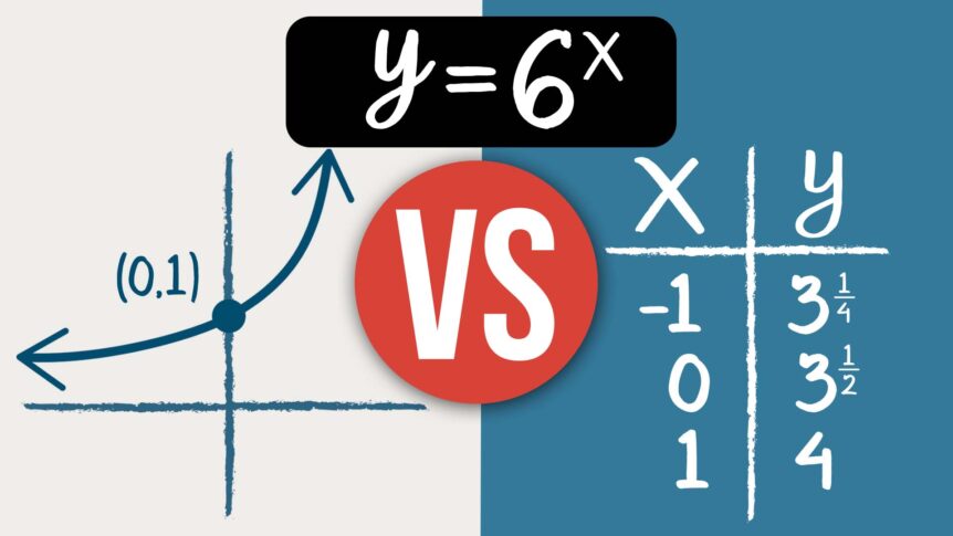
Okay. So this is a very intuitive way for you to understand using the graphing method. But now, what I want to do is show you a quicker, faster, easier way to understand exponential equations and be able to grab them. Okay. So now we have the general idea that we know if we ever get stuck or confused on graphing an exponential equation, we can always revert to the table formula. And I want you to remember that because it’s very helpful to be able to check your understanding or check data points on a graph using a table. But if we want to grab something and we want a quick way to understand what the graph looks like, it’s important to know two things. One, the parent graph, and two, the transformations. This is an exponential equation. The paragraph of an exponential equation looks just like this.
🎯Survive Math Class Checklist: Ten Steps to a Better Year: https://www.brianmclogan.com/email-ca
It doesn’t matter what the bases are, but as long as there are no transformations, we have a Y-intercept at zero, comma one, and a horizontal asymptote at zero. So you can see the domain is all real numbers, but the range is restricted from zero to Infinity. So now, what we need to do is understand our transformations. Now again, for any function, the transformations are going to affect the graph exactly the same. But the main thing we need to understand is whether we are applying transformations inside or outside the function. So we need to understand what exactly the function is for this exponential equation. And this exponential equation looks like y equals a base raised to the power X, where the input is the exponent. So if you recognize your transformation here when I am subtracting inside of the function because this is inside the exponent, when I do minus one, that will be shifting in the graph one unit to the right. When I add outside of the function, right, because this is not a part of this exponent, this is an outside function that will be a vertical shift, three units up.
You can make this same understanding by just looking at quadratics. If you remember y equals X squared, we did the same thing here. Y equals X squared. That graph looks something like this. If I subtract inside the equation and add three, that will affect the graph. Look at this. Y equals X minus one, quantity squared plus three. Notice how the one is inside and the three are outside. Now, what is this going to do to the quadratic? This will shift the graph one unit to the right and three units up. Now, what is it exactly? I moved the whole graph right. But specifically, I moved the Vertex right. I moved the lowest point on the graph. I shifted to over one unit and then up to three. So what are we going to want to move in this equation? The one point that we have for our parent graph Is the y-intercept.
So that’s exactly what I’m going to do. I’m just going to shift this graph one inch to the right and then three units up, and there goes, and gentlemen, that’s exactly what the graph looks like. It now has a y-intercept of one comma four, and then it has a horizontal asymptote here at three. The asymptote is not a part of the graph, but it is where the graph is approaching. So that’s why we do like to write that in with that dashed line. It’s also important to recognize that the domain has not been changed. It’s still all real numbers, and then the range will be from three to Infinity.
So there you have it. Lady. Gentlemen, I hope you found this post helpful. Check out the playlist and resources to see more examples of graphic exponential equations. Or look at the following video I have for you here.